Python数据分析:数据可视化实战教程( 二 )
#接下来 , 我们通过相关系数的大小来依次对特征进行可视化分析#首先 , 列出相关系数矩阵:df.corr()corrdf = Bikedata.corr()corrdf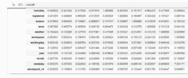 文章插图
文章插图
#各特征按照与租赁总量count的相关系数大小进行排序corrdf['count'].sort_values(ascending=False)count1.000000registered 0.966209casual 0.704764hour 0.405437temp 0.385954atemp 0.381967year 0.234959month 0.164673season 0.159801windspeed_rfr 0.111783windspeed 0.106074weekday 0.022602holiday 0.002978workingday -0.020764weather -0.127519humidity -0.317028Name: count, dtype: float64可见 , 特征对租赁总量的影响力为:
时段>温度>湿度>年份>月份>季节>天气>风速>工作日>节假日
对特征逐项分析
首先对时段进行分析
- 第一步
适合图形:因为湿度属于连续性数值变量 , 我们可以选择折线图反应变化趋势
- 第二步
应用函数:直接应用plt的plot函数即可完成折线图
figure,axes = plt.subplots(1,2,sharey=True)#设置一个1*2的画布 , 且共享y轴workingday_df.plot(figsize=(15,5),title='The average number of rentals initiated per hour in the working day',ax=axes[0])nworkingday_df.plot(figsize=(15,5),title='The average number of rentals initiated per hour in the nworking day',ax=axes[1])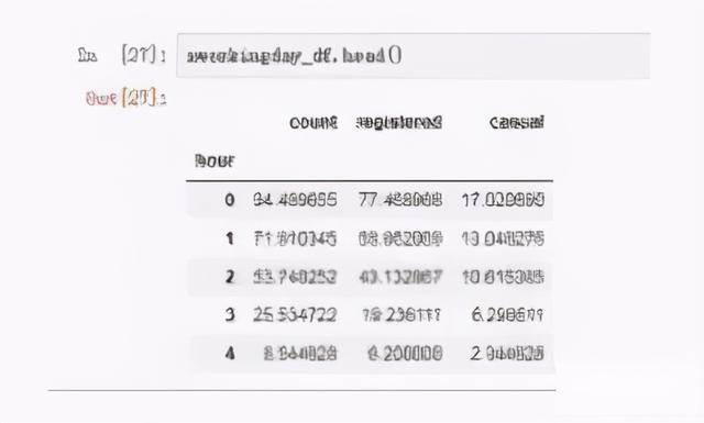 文章插图
文章插图- 第三步:设置参数
figure,axes = plt.subplots(1,2,sharey=True)#设置一个1*2的画布 , 且共享y轴workingday_df.plot(figsize=(15,5),title='The average number of rentals initiated per hour in the working day',ax=axes[0])nworkingday_df.plot(figsize=(15,5),title='The average number of rentals initiated per hour in the nworking day',ax=axes[1])可以看出:- 在工作日 , 会员出行对应两个很明显的早晚高峰期 , 并且在中午会有一个小的高峰 , 可能对应中午外出就餐需求;
- 工作日非会员用户出行高峰大概在下午三点;
- 工作日会员出行次数远多于非会员用户;
- 在周末 , 总体出行趋势一致 , 大部分用车发生在11-5点这段时间 , 早上五点为用车之最 。
- 第一步
适合图形:因为湿度属于连续性数值变量 , 我们可以选择折线图反应变化趋势
- 第二步
应用函数:直接应用plt的plot函数即可完成折线图
- 第三步
temp_df = Bikedata.groupby(['temp'],as_index='True').agg({'count':'mean','registered':'mean','casual':'mean'})temp_df.plot(title = 'The average number of rentals initiated per hour changes with the temperature')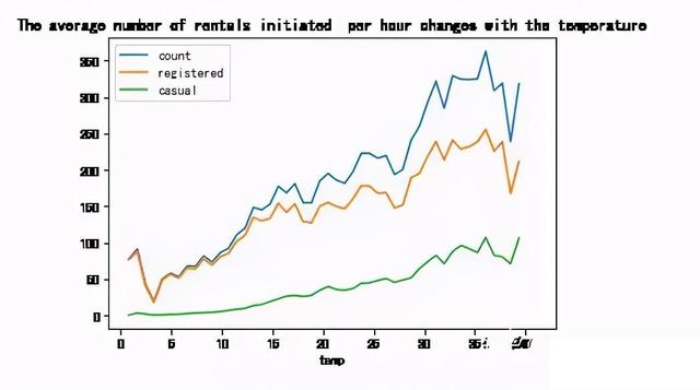 文章插图
文章插图
推荐阅读


![[绿豆]男人想要长寿,5件“耗阳”的事要“舍弃”,一些人表示很难做到](http://img88.010lm.com/img.php?https://image.uc.cn/s/wemedia/s/2020/26fa2bbcc60faf5ef39679c3f1999fd3.jpg)


- 西部数据在CES 2021推出多款4TB容量的旗舰级SSD
- WhatsApp收集用户数据新政惹众怒,“删除WhatsApp”在土耳其上热搜
- 计算机专业大一下学期,该选择学习Java还是Python
- 想自学Python来开发爬虫,需要按照哪几个阶段制定学习计划
- 未来想进入AI领域,该学习Python还是Java大数据开发
- 黑客窃取250万个人数据 意大利运营商提醒用户尽快更换SIM卡
- 阳狮报告:4成受访者认为自己的数据比免费服务更有价值
- 中消协点名大数据网络杀熟 反对利用消费者个人数据画像
- 学习大数据是否需要学习JavaEE
- 意大利运营商Ho Mobile被曝数据泄露