文章插图
文章插图
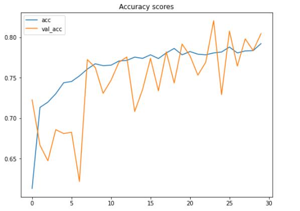
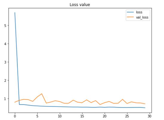
根据上面的两个图 ， 我们可以说 ， 即使在这30个时期内测试准确性和损失值都在波动 ， 模型的性能仍在不断提高 。
这里要注意的另一重要事情是 ， 由于我们在项目的早期应用了数据增强方法 ， 因此该模型不会遭受过拟合的困扰 。 我们在这里可以看到 ， 在最终迭代中 ， 训练和测试数据的准确性分别为79%和80% 。
有趣的事实：在实施数据增强方法之前 ， 我在训练数据上获得了100%的准确性 ， 在测试数据上获得了64%的准确性 ， 这显然是过拟合了 。 因此 ， 我们可以在此处清楚地看到 ， 增加训练数据对于提高测试准确性得分非常有效 ， 同时也可以减少过拟合 。
模型评估现在 ， 让我们深入了解使用混淆矩阵得出的测试数据的准确性 。 首先 ， 我们需要预测所有X_test并将结果从独热格式转换回其实际的分类标签 。
predictions = model.predict(X_test) predictions = one_hot_encoder.inverse_transform(predictions) 接下来 ， 我们可以像这样使用confusion_matrix()函数：
cm = confusion_matrix(y_test, predictions) 重要的是要注意函数中使用的参数是(实际值 ， 预测值) 。 该混淆矩阵函数的返回值是一个二维数组 ， 用于存储预测分布 。 为了使矩阵更易于解释 ， 我们可以使用Seaborn模块中的heatmap()函数进行显示 。 顺便说一句 ， 这里的类名列表的值是根据one_hotencoder.categories返回的顺序获取的 。
classnames = ['bacteria', 'normal', 'virus']plt.figure(figsize=(8,8)) plt.title('Confusion matrix') sns.heatmap(cm, cbar=False, xticklabels=classnames, yticklabels=classnames, fmt='d', annot=True, cmap=plt.cm.Blues) plt.xlabel('Predicted') plt.ylabel('Actual') plt.show()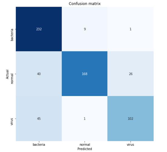
文章插图
根据上面的混淆矩阵 ， 我们可以看到45张病毒X射线图像被预测为细菌 。 这可能是因为很难区分这两种肺炎 。 但是 ， 至少因为我们对242个样本中的232个进行了正确分类 ， 所以我们的模型至少能够很好地预测由细菌引起的肺炎 。
这就是整个项目!谢谢阅读!下面是运行整个项目所需的所有代码 。
import os import cv2import pickle# Used to save variablesimport numpy as npimport matplotlib.pyplot as pltimport seaborn as snsfrom tqdm import tqdm# Used to display progress bar from sklearn.preprocessing import OneHotEncoder from sklearn.metrics import confusion_matrix from keras.models import Model, load_model from keras.layers import Dense, Input, Conv2D, MaxPool2D, Flatten from keras.preprocessing.image import ImageDataGenerator# Used to generate images np.random.seed(22) # Do not forget to include the last slashdef load_normal(norm_path):norm_files = np.array(os.listdir(norm_path))norm_labels = np.array(['normal']*len(norm_files))norm_images = []for image in tqdm(norm_files):# Read imageimage = cv2.imread(norm_path + image)# Resize image to 200x200 pximage = cv2.resize(image, dsize=(200,200))# Convert to grayscaleimage = cv2.cvtColor(image, cv2.COLOR_BGR2GRAY)norm_images.append(image)norm_images = np.array(norm_images)return norm_images, norm_labels def load_pneumonia(pneu_path):pneu_files = np.array(os.listdir(pneu_path))pneu_labels = np.array([pneu_file.split('_')[1] for pneu_file in pneu_files])pneu_images = []for image in tqdm(pneu_files):# Read imageimage = cv2.imread(pneu_path + image)# Resize image to 200x200 pximage = cv2.resize(image, dsize=(200,200))# Convert to grayscaleimage = cv2.cvtColor(image, cv2.COLOR_BGR2GRAY)pneu_images.append(image)pneu_images = np.array(pneu_images)return pneu_images, pneu_labels print('Loading images') # All images are stored in _images, all labels are in _labelsnorm_images, norm_labels = load_normal('/kaggle/input/chest-xray-pneumonia/chest_xray/train/NORMAL/') pneu_images, pneu_labels = load_pneumonia('/kaggle/input/chest-xray-pneumonia/chest_xray/train/PNEUMONIA/') # Put all train images to X_train X_train = np.append(norm_images, pneu_images, axis=0) # Put all train labels to y_trainy_train = np.append(norm_labels, pneu_labels) print(X_train.shape) print(y_train.shape) # Finding out the number of samples of each classprint(np.unique(y_train, return_counts=True))print('Display several images') fig, axes = plt.subplots(ncols=7, nrows=2, figsize=(16, 4)) indices = np.random.choice(len(X_train), 14) counter = 0 for i in range(2):for j in range(7):axes[i,j].set_title(y_train[indices[counter]])axes[i,j].imshow(X_train[indices[counter]], cmap='gray')axes[i,j].get_xaxis().set_visible(False)axes[i,j].get_yaxis().set_visible(False)counter += 1 plt.show()print('Loading test images') # Do the exact same thing as what we have done on train datanorm_images_test, norm_labels_test = load_normal('/kaggle/input/chest-xray-pneumonia/chest_xray/test/NORMAL/') pneu_images_test, pneu_labels_test = load_pneumonia('/kaggle/input/chest-xray-pneumonia/chest_xray/test/PNEUMONIA/') X_test = np.append(norm_images_test, pneu_images_test, axis=0) y_test = np.append(norm_labels_test, pneu_labels_test) # Save the loaded images to pickle file for future use with open('pneumonia_data.pickle', 'wb') as f:pickle.dump((X_train, X_test, y_train, y_test), f)# Here's how to load it with open('pneumonia_data.pickle', 'rb') as f:(X_train, X_test, y_train, y_test) = pickle.load(f) print('Label preprocessing') # Create new axis on all y data y_train = y_train[:, np.newaxis] y_test = y_test[:, np.newaxis] # Initialize OneHotEncoder object one_hot_encoder = OneHotEncoder(sparse=False) # Convert all labels to one-hot y_train_one_hot = one_hot_encoder.fit_transform(y_train) y_test_one_hot = one_hot_encoder.transform(y_test) print('Reshaping X data') # Reshape the data into (no of samples, height, width, 1), where 1 represents a single color channel X_train = X_train.reshape(X_train.shape[0], X_train.shape[1], X_train.shape[2], 1) X_test = X_test.reshape(X_test.shape[0], X_test.shape[1], X_test.shape[2], 1) print('Data augmentation') # Generate new images with some randomness datagen = ImageDataGenerator(rotation_range = 10,zoom_range = 0.1,width_shift_range = 0.1,height_shift_range = 0.1) datagen.fit(X_train) train_gen = datagen.flow(X_train, y_train_one_hot, batch_size = 32) print('CNN') # Define the input shape of the neural network input_shape = (X_train.shape[1], X_train.shape[2], 1) print(input_shape) input1 = Input(shape=input_shape) cnn = Conv2D(16, (3, 3), activation='relu', strides=(1, 1),padding='same')(input1) cnn = Conv2D(32, (3, 3), activation='relu', strides=(1, 1),padding='same')(cnn) cnn = MaxPool2D((2, 2))(cnn) cnn = Conv2D(16, (2, 2), activation='relu', strides=(1, 1),padding='same')(cnn) cnn = Conv2D(32, (2, 2), activation='relu', strides=(1, 1),padding='same')(cnn) cnn = MaxPool2D((2, 2))(cnn) cnn = Flatten()(cnn) cnn = Dense(100, activation='relu')(cnn) cnn = Dense(50, activation='relu')(cnn) output1 = Dense(3, activation='softmax')(cnn) model = Model(inputs=input1, outputs=output1) model.compile(loss='categorical_crossentropy',optimizer='adam', metrics=['acc']) # Using fit_generator() instead of fit() because we are going to use data # taken from the generator. Note that the randomness is changing # on each epoch history = model.fit_generator(train_gen, epochs=30,validation_data=http://kandian.youth.cn/index/(X_test, y_test_one_hot)) # Saving model model.save('pneumonia_cnn.h5') print('Displaying accuracy') plt.figure(figsize=(8,6)) plt.title('Accuracy scores') plt.plot(history.history['acc']) plt.plot(history.history['val_acc']) plt.legend(['acc', 'val_acc']) plt.show() print('Displaying loss') plt.figure(figsize=(8,6)) plt.title('Loss value') plt.plot(history.history['loss']) plt.plot(history.history['val_loss']) plt.legend(['loss', 'val_loss']) plt.show() # Predicting test data predictions = model.predict(X_test) print(predictions) predictions = one_hot_encoder.inverse_transform(predictions) print('Model evaluation') print(one_hot_encoder.categories_) classnames = ['bacteria', 'normal', 'virus'] # Display confusion matrix cm = confusion_matrix(y_test, predictions) plt.figure(figsize=(8,8)) plt.title('Confusion matrix') sns.heatmap(cm, cbar=False, xticklabels=classnames, yticklabels=classnames, fmt='d', annot=True, cmap=plt.cm.Blues) plt.xlabel('Predicted') plt.ylabel('Actual') plt.show()